Fine-Tuning: QLoRA

The goal of this post is to demonstrate how to fine-tune an LLM (Llama-3.1-8B-Instruct) using QLoRA to solve a classic machine learning task: classifying emails as spam or not spam. If you haven’t read the previous post on fine-tuning yet, I highly recommend doing so, as it covers the foundational concepts, approaches, parameters, and other essential details.

The topics covered in this post include:

Understanding QLoRA
Data Preprocessing
Inference without Fine-Tuning
Fine-Tuning: Hyperparameter Adjustment
Fine-Tuning: Training
Inference of the Tuned Model

Each script presented here was executed in Google Colab. Except for the data preprocessing step, all fine-tuning stages were run in separate notebooks, where I also outline the configuration used.

Understanding QLoRA

Quantized Low-Rank Adaptation (QLoRA) combines the ideas of quantization and LoRA to significantly reduce memory usage during LLM fine-tuning, without sacrificing performance.

Quantization is a technique used to reduce the numerical precision of a model’s parameters. Imagine that you need to load a 7-billion-parameter LLM, but your hardware resources are limited, this quickly becomes impractical. Even using a cloud machine can lead to high costs. With quantization, instead of using the model’s original 32-bit weights, they are converted to 16-bit, 8-bit, or even lower-precision representations. This reduces the model size, can speed up computation, and in most cases still preserves acceptable performance.

Numbers are stored in memory using 3 components: the sign, mantissa, and exponent. The sign indicates whether the value is positive or negative. The exponent defines the power of two, allowing the number to be represented at different scales. The mantissa determines how precise the value will be. Below, I show how these components are represented in both the float32 and float16 formats. Typically, float32 allocates 1 bit for the sign, 8 bits for the exponent, and 23 bits for the mantissa, while float16 uses 1 bit for the sign, 5 bits for the exponent, and 10 bits for the mantissa.

Now imagine that we want to convert a weight matrix in the range [−1000, 1000], originally stored in 32 bits, into uint8 values, which range from [0, 255]. To perform this transformation, we first compute the scale, which adjusts the amplitude of the real values so they fit within the target interval. Next, we calculate the zero point, which ensures the original values are aligned with the lower bound of the new range. Finally, to obtain the quantized value, we divide the original value by the scale, add the zero point, and round the result to the nearest integer.

scale = (x_max − x_min) / (q_max − q_min)

zero_point = round(q_min − x_min / scale)

x_quantized = round(x / scale + zero_point)

Note: Values prefixed with x refer to the original range, while values prefixed with q correspond to the target range.

Below is the formula used to dequantize the value, meaning to recover an approximation of the original real number. It is important to note that this process introduces a loss of precision, so the reconstructed value typically does not match the original exactly.

x ≈ (q − zero_point) * scale

To make the process clearer, let’s quantize 3 example values: –1000, 100, and 1000. See the demonstration below:

scale = (1000 - (-1000)) / (255 - 0) ~= 7.84314
zero_point = round(0 - (-1000) / 7.84314)  = 127

# -1000
x_quantized = round(-1000 / 7.84314 + 127) = 0
x_dequantized = (0 - 127) * 7.84314 ~= -996.079

# 100
x_quantized = round(100 / 7.84314 + 127) =141
x_dequantized = (141 - 127) * 7.84314 ~= 101.961

# 1000
x_quantized = round(1000 / 7.84314 + 127) =255
x_dequantized = (255 - 127) * 7.84314 ~= 996.079

Note that this is just one way to perform quantization. Other approaches are also possible.

LoRA (Low-Rank Adaptation), on the other hand, aims to reduce the number of parameters that need to be trained by applying a low-rank matrix decomposition. In this context, the rank represents how many independent rows or columns a matrix truly has, that is, its essential complexity. This allows a large matrix to be approximated by the multiplication of 2 smaller matrices. Below, I show an example where a 4×4 matrix is represented using 2 smaller matrices: one of size 4×1 and the other of size 1×4.

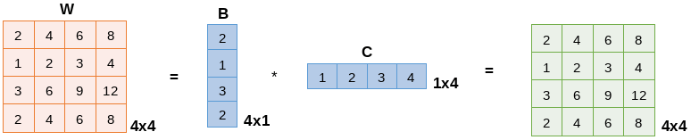
Following this principle, the goal of LoRA is to generate a matrix ΔW = BA that is much smaller than the original weight matrix W. In the example above, W has a 4×4 shape, totaling 16 values, while ΔW contains only 8 parameters: 4×1 from matrix B and 1×4 from matrix A. Now imagine applying this idea at scale, in language models with billions or even trillions of parameters. The reduction in the number of trainable parameters becomes massive. Thus, when using LoRA, the final adjusted matrix becomes W’ = W + ΔW. In other words, the model does not update W directly, it only learns ΔW, which is much smaller and far easier to train.

In summary, QLoRA significantly reduces the memory required to fine-tune an LLM without sacrificing performance. It is one of the most effective techniques available today for environments with limited computational resources, such as mobile devices or embedded systems. However, some challenges remain, including finding the right balance between efficiency and quality, as well as properly tuning the hyperparameters (both those of the model and those specific to QLoRA). If you want to explore the topic further, click here to access the QLoRA paper.

Data Preprocessing

As mentioned at the beginning of this post, I highly recommend reading the previous one, where I provide a more detailed explanation of the parameters and code used. Additionally, since this data preprocessing step will be executed in every notebook, there is no need to include the notebook configuration in this section.

For context, the dataset used (from Kaggle) addresses a classic problem: classifying emails as spam or not spam. Below, I present the data preprocessing steps applied.

from datasets import load_dataset, DatasetDict, ClassLabel

data = load_dataset("csv", data_files="emails.csv", delimiter=",")

labels = ClassLabel(
    num_classes=2,
    names=["Not Spam", "Spam"]
)
data = data.cast_column("spam", labels)

split = data["train"].train_test_split(
    test_size=0.2,
    seed=42,
    stratify_by_column="spam"
)
train_data, val_data = split["train"], split["test"]

split = val_data.train_test_split(
    test_size=0.5,
    seed=42,
    stratify_by_column="spam"
)
val_data, test_data = split["train"], split["test"]

data = DatasetDict({
    "train": train_data,
    "val": val_data,
    "test": test_data
})

The dataset was split into training, validation, and test sets with an 80/10/10 distribution. Since it is an imbalanced dataset, containing far more non-spam examples than spam, the split was performed using stratification, ensuring that the class proportions remain consistent across all subsets. See the dataset below:

DatasetDict({
    train: Dataset({
        features: ['text', 'spam'],
        num_rows: 4582
    })
    val: Dataset({
        features: ['text', 'spam'],
        num_rows: 573
    })
    test: Dataset({
        features: ['text', 'spam'],
        num_rows: 573
    })
})

Additionally, to verify the class distribution in each split, you can run:

from numpy import unique

unique(data["train"]["spam"], return_counts=True)
unique(data["val"]["spam"], return_counts=True)
unique(data["test"]["spam"], return_counts=True)

The result is:

(array([0, 1]), array([3488, 1094]))  # train
(array([0, 1]), array([436, 137]))  # val
(array([0, 1]), array([436, 137]))  # test

Inference without Fine-Tuning

The goal of this section is to use the Llama-3.1-8B-Instruct model without any fine-tuning. In the previous post, I used Phi-2 in both its base version and its classification variant. In this post, however, I will use only the base version, as it naturally delivers better performance.

To run the inference with Llama, I used an L4 GPU with high RAM capacity on Google Colab. Additionally, to access the Llama-3.1-8B-Instruct model, you need to submit a request through your Hugging Face account. Once your access is approved (you will receive an email notification), you must load your Hugging Face token before initializing the model. In my case, I stored the token as an environment variable inside a .env file, which I loaded in Colab:

HF_TOKEN="your-token"

Then, I simply loaded the variables using:

from dotenv import load_dotenv
load_dotenv()

Below is the code used to load the model.

from transformers import AutoModelForCausalLM, AutoTokenizer, pipeline
import torch

tokenizer = AutoTokenizer.from_pretrained("meta-llama/Llama-3.1-8B-Instruct")
if tokenizer.pad_token is None:
  tokenizer.pad_token = tokenizer.eos_token

model = AutoModelForCausalLM.from_pretrained(
    "meta-llama/Llama-3.1-8B-Instruct",
    dtype=torch.float16,
    device_map="auto"
)

pipe = pipeline(
    "text-generation",
    model=model,
    tokenizer=tokenizer,
    model_kwargs={
        "max_new_tokens": 10,
        "return_full_text": False,
        "temperature": 0.1,
        "do_sample": True
    }
)

Unlike the previous post, here I used the Hugging Face pipeline, which abstracts the entire process of text preprocessing, generation, and post-processing. Within this pipeline, you specify the task type (in this case, “text-generation”), as well as the model and tokenizer. In addition, a few important parameters were included in model_kwargs:

max_new_tokens: the maximum number of tokens the model can generate in the output.
temperature: controls the randomness of the generation. Lower values make the output more deterministic.
do_sample: enables or disables sampling during text generation. When True, the model samples tokens based on their probabilities, adding an element of randomness. When False, it always selects the most likely token.
return_full_text: when False, only the generated text is returned, without repeating the input prompt.

To assess the model’s effectiveness, we used the test set. In the code below, the classify_text function is responsible for classifying the input text passed as a argument. Note that a simple prompt was created to instruct the model about the task. The messages in chat format (system + user) are then sent to the pipeline. Finally, the function returns the output generated by the model.

def classify_text(text):

  prompt = (
      "You are a text classification model.\n"
      "Classify the following text as 'Spam' or 'Not Spam'.\n"
      "Return ONLY one of these two words."
  )

  messages = [
      {"role": "system", "content": prompt},
      {"role": "user", "content": text},
  ]

  outputs = pipe(messages)

  return outputs[0]["generated_text"][-1]["content"]

Below is the usage of the function above to classify each text/email from the test set.

responses, predictions = [], []

for i, text in enumerate(data["test"]["text"]):
    print(f"\r{i}", end="")

    resp = classify_text(text)

    if "not spam" in resp.lower():
        pred = 0
    else:
        if "spam" in resp.lower():
            pred = 1
        else:
            pred = 0

    responses.append(resp)
    predictions.append(pred)

To evaluate the results of this type of problem, the most suitable metric is precision, since the dataset is imbalanced and false positives, i.e., emails classified as spam when they are not, are the most critical errors in this scenario. Still, to obtain a more complete view, it is recommended to look at other metrics as well, such as accuracy, recall, and F1-score, as they are easy to interpret and have low computational cost.

To provide better context, here is a simple explanation of each metric (I will write a more detailed post about them in the future):

accuracy: percentage of correct predictions. Works best when the classes are balanced. Formula: (TP + TN) / (TP + TN + FP + FN).
precision: indicates how many of the predicted positives are actually positive. Useful when the dataset is imbalanced and false positives carry more weight. Formula: TP / (TP + FP).
recall: measures how many of the actual positives the model successfully identified. Important when false negatives are more critical. Formula: TP / (TP + FN).
F1-score: harmonic mean between precision and recall. Useful for imbalanced datasets and when both metrics need to be balanced. Formula: 2 * (precision * recall) / (precision + recall).
Note: TP = True Positive, TN = True Negative, FP = False Positive, and FN = False Negative.

The code below computes the metrics described above for the model used.

!pip install -q evaluate

import evaluate

f1 = evaluate.load("f1")
precision = evaluate.load("precision")
recall = evaluate.load("recall")
roc_auc = evaluate.load("roc_auc")
accuracy = evaluate.load("accuracy")

metrics = {
    "f1": f1.compute(predictions=predictions, references=data["test"]["spam"])["f1"],
    "precision": precision.compute(predictions=predictions, references=data["test"]["spam"])["precision"],
    "recall": recall.compute(predictions=predictions, references=data["test"]["spam"])["recall"],
    "auc": roc_auc.compute(prediction_scores=predictions, references=data["test"]["spam"])["roc_auc"],
    "accuracy": accuracy.compute(predictions=predictions, references=data["test"]["spam"])["accuracy"]
}

Here is the result, where the model achieved 60% precision:

{'f1': 0.7430167597765364,
 'precision': 0.6018099547511312,
 'recall': 0.9708029197080292,
 'auc': np.float64(0.884484028661354),
 'accuracy': 0.8394415357766143}

Fine-Tuning: Hyperparameter Adjustment

The goal of this section is to optimize the model’s hyperparameters, meaning to find a set of values that improves its performance. Some of the parameters used here were already discussed in the previous post, so I will not go over those details again.

For this step, I used an A4 GPU with high RAM on Google Colab.

Below is the code used to load the model:

!pip install -q bitsandbytes

from transformers import AutoTokenizer, AutoModelForSequenceClassification, DataCollatorWithPadding, BitsAndBytesConfig
import torch

tokenizer = AutoTokenizer.from_pretrained("meta-llama/Llama-3.1-8B-Instruct")
if tokenizer.pad_token is None:
  tokenizer.pad_token = tokenizer.eos_token
data_collator = DataCollatorWithPadding(tokenizer=tokenizer)

def model_init():

  id2label = {0: "Not Spam", 1: "Spam"}
  label2id = {"Not Spam": 0, "Spam": 1}

  quantization_config = BitsAndBytesConfig(
      load_in_4bit=True,
      bnb_4bit_compute_dtype=torch.float16,
      bnb_4bit_quant_type="nf4",
      bnb_4bit_use_double_quant=True,
      llm_int8_enable_fp32_cpu_offload=True
  )

  model = AutoModelForSequenceClassification.from_pretrained(
      "meta-llama/Llama-3.1-8B-Instruct",
      quantization_config=quantization_config,
      num_labels=2,
      id2label=id2label,
      label2id=label2id,
      pad_token_id=tokenizer.pad_token_id
  )

  for param in model.parameters():
    param.requires_grad = False

  return model

Note that the model was wrapped inside a function. Since the hyperparameters will be optimized, the model needs to be reloaded at each execution. This is required because the approach used here is random search, where the experiments are run N times (with N defined by the user).

In addition, the model will be loaded in 4-bit quantized format using the bitsandbytes library. The following configurations come from the BitsAndBytesConfig class:

load_in_4bit: specifies whether 4-bit quantization should be used.
bnb_4bit_compute_dtype: data type used for computations during training when 4-bit quantization is active. It is typically chosen to balance computational efficiency and numerical precision.
bnb_4bit_quant_type: defines how values are represented after quantization. The "nf4" option refers to the NormalFloat4 format introduced in the QLoRA paper. It is based on the idea that many neural network weights follow an approximately normal distribution. Instead of uniformly spaced levels, NF4 allocates more resolution where the values are more frequent (near zero), reducing quantization error and better preserving model quality.
bnb_4bit_use_double_quant: when set to True, enables an additional quantization step (double quantization) applied to scale factors or quantization constants associated with the 4-bit weights. For example, after quantizing a weight to 4 bits, a scale factor stored in 16 bits may still be needed. With double quantization, this factor is quantized as well (e.g., to 8 bits), further reducing the required storage. This yields an additional ~0.4 bits per parameter of savings, at the cost of slightly increased loading and processing complexity.
llm_int8_enable_fp32_cpu_offload: offloads part of the computation to the CPU in FP32 mode when necessary.

Additionally, it is important to note that all original model parameters were frozen (requires_grad = False), as only the LoRA adapters will be trained.

Before optimizing the hyperparameters, one more step is required. Since the dataset is imbalanced, training it directly would make the model favor the majority class, in this case, non-spam emails. To mitigate this, we apply data augmentation, a technique that generates new samples from existing ones by applying small transformations that preserve the original meaning. The goal is to increase dataset diversity without collecting new data. To balance the dataset, augmentation was applied only to the training split and exclusively to examples from the “Spam” class. In the code below, this step is performed before the train/validation/test split, and afterward the data is reorganized into a DatasetDict.

!pip install -q nlpaug

import nlpaug.augmenter.word as naw
import nltk
from random import choice
from datasets import Dataset, concatenate_datasets

def augment_data(train_data):
  augmentation = naw.SynonymAug(aug_src='wordnet')

  spam = train_data.filter(lambda x: x["spam"] == 1)
  not_spam = train_data.filter(lambda x: x["spam"] == 0)

  augmented_texts = []
  for i in range(2):
    augmented_texts += [augmentation.augment(text)[0] for text in spam["text"]]

  rest = len(not_spam) - (len(augmented_texts) + len(spam))
  augmented_texts += [augmentation.augment(choice(spam["text"]))[0] for _ in range(rest)]

  augmented_dataset = Dataset.from_dict({
      "text": augmented_texts,
      "spam": [1] * len(augmented_texts)
  })
  augmented_dataset = augmented_dataset.cast_column("spam", labels)

  train_data = concatenate_datasets([train_data, augmented_dataset])

  return train_data

train_data = augment_data(train_data)

Below is the explanation of the code:

naw.SynonymAug(aug_src='wordnet'): augmentation generator that replaces words with synonyms using WordNet.
For loop: creates 2 variations for each spam sentence. This factor of 2 was chosen to increase the minority class without exceeding the number of non-spam samples.
rest and augmented_texts: if additional samples are needed to fully balance the dataset, new sentences are generated using randomly selected spam examples as the base.
augmented_dataset: dataset containing only the sentences created through augmentation, all labeled as spam.
concatenate_datasets: merges the original training dataset with the augmented one, ensuring the final class balance.

To make the process clearer, here is a simple example of a sentence transformed by the augmentation step:

augmentation = naw.SynonymAug(aug_src='wordnet')
augmentation.augment("I like going to the gym whenever possible.")[0]
# Result: I wish going to the gymnasium whenever possible.

With this, when checking the number of unique classes in each split, we see that the training data is balanced, while the validation and test sets remain imbalanced, which is desirable, as it preserves the real-world characteristics of the dataset during model evaluation.

(array([0, 1]), array([3488, 3488]))  # train
(array([0, 1]), array([436, 137])),  # val
(array([0, 1]), array([436, 137]))  # test

To complete the data preprocessing before running the random search, the code below generates the prompt that will be passed to the model and performs text tokenization, along with label creation. This ensures that the model receives the data in the correct format for training.

def preprocessing(data):

  prefix = "Classify the following text as 'Spam' or 'Not Spam': "
  data["text"] = [prefix + text if text is not None else "" for text in data["text"]]

  encoding = tokenizer(
      text=data["text"],
      truncation=True,
      max_length=128
  )

  encoding["labels"] = data["spam"]

  return encoding

data = data.map(preprocessing, batched=True)

Thus, the dataset takes on the following format:

DatasetDict({
    train: Dataset({
        features: ['text', 'spam', 'input_ids', 'attention_mask', 'labels'],
        num_rows: 6976
    })
    val: Dataset({
        features: ['text', 'spam', 'input_ids', 'attention_mask', 'labels'],
        num_rows: 573
    })
    test: Dataset({
        features: ['text', 'spam', 'input_ids', 'attention_mask', 'labels'],
        num_rows: 573
    })
})

Finally, the random search can be performed:

# ==== Random Search ====
class BinaryClassificationRandomSearch:

  def __init__(self, model_init, tokenizer, data_collator, hyperparameters):

    self.__model_init = model_init
    self.__tokenizer = tokenizer
    self.__data_collator = data_collator

    self.__hyperparameters = hyperparameters

    self.__f1 = evaluate.load("f1")
    self.__precision = evaluate.load("precision")
    self.__recall = evaluate.load("recall")
    self.__roc_auc = evaluate.load("roc_auc")
    self.__accuracy = evaluate.load("accuracy")

    self.df = DataFrame()


  def run(self, data, total_executions, epochs):

    for execution in range(total_executions):
      print(f"Execution: {execution + 1}")

      self.__get_hyperparameters()

      self.__train(data, epochs)

      self.__metrics()

      self.__concat_dataframe()

      del self.__trainer
      torch.cuda.empty_cache()
      gc.collect()

    return self.df


  def __get_hyperparameters(self):

    seed()

    self.__lr = uniform(*self.__hyperparameters["learning_rate"])
    self.__lr_scheduler_type = choice(self.__hyperparameters["lr_scheduler_type"])
    self.__weight_decay = uniform(*self.__hyperparameters["weight_decay"])
    self.__warmup_ratio = uniform(*self.__hyperparameters["warmup_ratio"])
    self.__per_device_train_batch_size = randint(*self.__hyperparameters["per_device_train_batch_size"])

    # LoRA hyperparameters
    self.__r = randint(*self.__hyperparameters["r"])
    self.__lora_alpha = randint(*self.__hyperparameters["lora_alpha"])
    self.__lora_dropout = uniform(*self.__hyperparameters["lora_dropout"])


  def __train(self, data, epochs):

    training_args = TrainingArguments(
      learning_rate=self.__lr,
      lr_scheduler_type=self.__lr_scheduler_type,
      weight_decay=self.__weight_decay,
      warmup_ratio=self.__warmup_ratio,
      per_device_train_batch_size=self.__per_device_train_batch_size,
      per_device_eval_batch_size=8,
      num_train_epochs=epochs,
      eval_strategy="epoch",
      group_by_length = True,
      push_to_hub=False,
      report_to=[],
      disable_tqdm=True
    )

    model = self.__model_init()
    config = LoraConfig(
        r = self.__r,
        lora_alpha = self.__lora_alpha,
        lora_dropout = self.__lora_dropout,
        bias = "none",
        task_type = "SEQ_CLS"
    )
    model = get_peft_model(model, config)

    self.__trainer = Trainer(
      model=model,
      args=training_args,
      train_dataset=data["train"],
      eval_dataset={"Training": data["train"], "Validation": data["val"]},
      processing_class=self.__tokenizer,
      data_collator=self.__data_collator,
      compute_metrics=self.__compute_metrics
    )

    self.__trainer.train()


  def __metrics(self):

    self.__f1_train, self.__precision_train, self.__recall_train, self.__auc_train, self.__acc_train = None, None, None, None, None
    self.__f1_val, self.__precision_val, self.__recall_val, self.__auc_val, self.__acc_val = None, None, None, None, None

    for i in range(len(self.__trainer.state.log_history) -1, -1, -1):
      if "eval_Training_runtime" in self.__trainer.state.log_history[i]:
        self.__f1_train = self.__trainer.state.log_history[i]["eval_Training_f1"]
        self.__precision_train = self.__trainer.state.log_history[i]["eval_Training_precision"]
        self.__recall_train = self.__trainer.state.log_history[i]["eval_Training_recall"]
        self.__auc_train = self.__trainer.state.log_history[i]["eval_Training_auc"]
        self.__acc_train = self.__trainer.state.log_history[i]["eval_Training_accuracy"]

      if "eval_Validation_runtime" in self.__trainer.state.log_history[i]:
        self.__f1_val = self.__trainer.state.log_history[i]["eval_Validation_f1"]
        self.__precision_val = self.__trainer.state.log_history[i]["eval_Validation_precision"]
        self.__recall_val = self.__trainer.state.log_history[i]["eval_Validation_recall"]
        self.__auc_val = self.__trainer.state.log_history[i]["eval_Validation_auc"]
        self.__acc_val = self.__trainer.state.log_history[i]["eval_Validation_accuracy"]

      if self.__f1_train and self.__f1_val:
        break


  def __concat_dataframe(self):

    self.df = concat([
      self.df,
      DataFrame({
        "learning_rate": self.__lr,
        "lr_scheduler_type": self.__lr_scheduler_type,
        "weight_decay": self.__weight_decay,
        "warmup_ratio": self.__warmup_ratio,
        "per_device_train_batch_size": self.__per_device_train_batch_size,
        "r": self.__r,
        "lora_alpha": self.__lora_alpha,
        "lora_dropout": self.__lora_dropout,
        "f1_train": self.__f1_train,
        "f1_val": self.__f1_val,
        "precision_train": self.__precision_train,
        "precision_val": self.__precision_val,
        "recall_train": self.__recall_train,
        "recall_val": self.__recall_val,
        "auc_train": self.__auc_train,
        "auc_val": self.__auc_val,
        "acc_train": self.__acc_train,
        "acc_val": self.__acc_val,
      }, index=[0])
    ], ignore_index=True)


  def __compute_metrics(self, eval_pred):

    predictions, labels = eval_pred
    label_predictions = argmax(predictions, axis=1)

    metrics = {
        "f1": self.__f1.compute(predictions=label_predictions, references=labels)["f1"],
        "precision": self.__precision.compute(predictions=label_predictions, references=labels)["precision"],
        "recall": self.__recall.compute(predictions=label_predictions, references=labels)["recall"],
        "auc": self.__roc_auc.compute(prediction_scores=predictions[:, 1], references=labels)["roc_auc"],
        "accuracy": self.__accuracy.compute(predictions=label_predictions, references=labels)["accuracy"]
    }

    return metrics

Most of this code was already explained in the previous post; therefore, the explanation here will focus only on the LoRA components:

First, the LoRA configuration (LoraConfig) is created
- r: the rank of the matrix decomposition. It controls the size of the low-rank matrices to be learned, reducing computational complexity and the number of trainable parameters. For example, consider a 1000×1000 weight matrix: with r = 4, it is approximated by a 1000×4 and a 4×1000 matrix. Instead of training 1,000,000 parameters, we now train only 8,000.
- lora_alpha: the scaling factor that determines how much of the LoRA update is added to the original weights. The update has the form: ΔW = (lora_alpha / r) · (B A), enabling fine-grained control over the magnitude of weight updates.
- lora_dropout: dropout percentage applied only to the LoRA modules, helping prevent overfitting. Similar to standard neural networks, randomly disabling some activations prevents the model from becoming too dependent on specific training patterns. For instance, with a value of 0.2, 20% of the LoRA weights will be randomly disabled during training.
- bias: defines whether bias terms will be trained in the LoRA modules. Bias adds a constant value to the output of a layer and can help the model adapt to data. With bias="none", the biases remain frozen — the most common approach in LoRA.
- task_type="SEQ_CLS": specifies that the task is sequence classification.
Next, the configuration is applied to the model using get_peft_model: After defining the configuration, this function converts the original model into a PEFT (Parameter-Efficient Fine-Tuning) model by inserting the LoRA modules into its layers. In practice, this means that only the LoRA matrices (BA) are trained, while the original model weights remain frozen.

Below is the code used to actually run the random search, which was executed 10 times with 3 epochs in each run:

hyperparameters = {
    "learning_rate": [1e-6, 1e-3],
    "lr_scheduler_type": ["linear", "cosine"],
    "weight_decay": [1e-2, 1e-4],
    "warmup_ratio": [0, 0.1],
    "per_device_train_batch_size": [4, 64],
    "r": [4, 32],
    "lora_alpha": [4, 64],
    "lora_dropout": [0, 1]
}

random_search = BinaryClassificationRandomSearch(
    model_init=model_init,
    tokenizer=tokenizer,
    data_collator=data_collator,
    hyperparameters=hyperparameters
)

df = random_search.run(
    data=data,
    total_executions=10,
    epochs=3
)

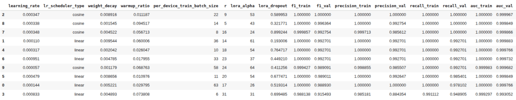
Below are the results of the 10 random search runs. To display the dataframe in the same order as shown in the image, use: df.sort_values(["f1_val", "precision_val"], ascending=False). The chosen hyperparameter configuration was the first one, as it delivered excellent results, reaching 100% precision with no signs of overfitting. It is worth noting that such high results may seem “too good,” but it’s important to remember that an LLM is inherently powerful and, when fine-tuned on a relatively simple dataset like this one, it is expected to perform extremely well.

Fine-Tuning: Training

To run this step on Google Colab, I used a notebook with an L4 GPU and high RAM. As in the previous sections, the training parameters were explained in more detail in the previous post.

The dataset processing is the same as in the hyperparameter optimization section, including the augmentation step used to balance the training data. The metrics used to evaluate the models remain the same, with particular emphasis on precision, which is the most relevant metric for the problem at hand. Additionally, since we need to load the LoRA parameters with the selected configuration, the following code handles this process:

from transformers import AutoTokenizer, AutoModelForSequenceClassification, DataCollatorWithPadding, BitsAndBytesConfig
import torch
from peft import LoraConfig, get_peft_model

tokenizer = AutoTokenizer.from_pretrained("meta-llama/Llama-3.1-8B-Instruct")
if tokenizer.pad_token is None:
  tokenizer.pad_token = tokenizer.eos_token
data_collator = DataCollatorWithPadding(tokenizer=tokenizer)

def model_init():

  id2label = {0: "Not Spam", 1: "Spam"}
  label2id = {"Not Spam": 0, "Spam": 1}

  quantization_config = BitsAndBytesConfig(
      load_in_4bit=True,
      bnb_4bit_compute_dtype=torch.float16,
      bnb_4bit_quant_type="nf4",
      bnb_4bit_use_double_quant=True,
      llm_int8_enable_fp32_cpu_offload=True
  )

  model = AutoModelForSequenceClassification.from_pretrained(
      "meta-llama/Llama-3.1-8B-Instruct",
      quantization_config=quantization_config,
      num_labels=2,
      id2label=id2label,
      label2id=label2id,
      pad_token_id=tokenizer.pad_token_id
  )

  for param in model.parameters():
    param.requires_grad = False

  return model

model = model_init()

config = LoraConfig(
    r = 9,
    lora_alpha = 53,
    lora_dropout = 0.589953,
    bias = "none",
    task_type = "SEQ_CLS"
)

model = get_peft_model(model, config)

As mentioned earlier in this post, when using LoRA and freezing all original model parameters, only the LoRA parameters are actually updated during training. With the selected configuration, this results in 3,842,048 trainable parameters, while 4,015,271,936 remain frozen, meaning that only about 0.1% of the model’s parameters are being trained. To view this calculation, use the code below:

trainable = sum(param.numel() for param in model.parameters() if param.requires_grad)
frozen = sum(param.numel() for param in model.parameters() if not param.requires_grad)
print(f"Trainable: {trainable:,} | Frozen: {frozen:,}")

To use the hyperparameters selected during the random search, run the code below. Note that the training will be performed for 5 epochs.

from transformers import TrainingArguments

training_args = TrainingArguments(
    learning_rate=0.000347,
    lr_scheduler_type="cosine",
    weight_decay=0.008916,
    warmup_ratio=0.011187,
    per_device_train_batch_size=22,
    per_device_eval_batch_size=8,
    num_train_epochs=5,
    eval_strategy="epoch",
    group_by_length = True,
    output_dir="llama-3.1-spam-vs-no-spam-classification",
    save_strategy="epoch",
    save_total_limit=3,
    push_to_hub=False,
    hub_model_id="edvaldomelo/llama-3.1-spam-vs-no-spam-classification",
    report_to=[]
)

To actually train the model, run:

from transformers import Trainer

trainer = Trainer(
    model=model,
    args=training_args,
    train_dataset=data["train"],
    eval_dataset={"train": data["train"], "val": data["val"]},
    processing_class=tokenizer,
    data_collator=data_collator,
    compute_metrics=compute_metrics
)

trainer.train()

Below are the training results for each epoch:

To perform the final evaluation of the model, I used the test dataset:

trainer.evaluate(eval_dataset=data["test"])

On this test dataset, the model achieved 100% precision and 99% F1-score, which is very close to the results obtained on the validation set and significantly better than the performance of the model without fine-tuning, which reached 60% precision and 74% F1-score.

Finally, the model was uploaded to the Hugging Face Hub for inference:

trainer.push_to_hub()
tokenizer.push_to_hub("edvaldomelo/llama-3.1-spam-vs-no-spam-classification")

Inference of the Tuned Model

The goal of this section is to use the model that was trained and uploaded to the Hugging Face Hub. For this step, a notebook with an L4 GPU and high RAM was used.

To load the model, use the code below.

from transformers import AutoTokenizer, AutoModelForSequenceClassification

tokenizer = AutoTokenizer.from_pretrained("edvaldomelo/llama-3.1-spam-vs-no-spam-classification")
if tokenizer.pad_token is None:
  tokenizer.pad_token = tokenizer.eos_token

id2label = {0: "Not Spam", 1: "Spam"}
label2id = {"Not Spam": 0, "Spam": 1}

model = AutoModelForSequenceClassification.from_pretrained(
    "edvaldomelo/llama-3.1-spam-vs-no-spam-classification",
    num_labels=2,
    id2label=id2label,
    label2id=label2id,
    pad_token_id=tokenizer.pad_token_id
)

To evaluate the model, a synthetic dataset was created using ChatGPT, containing 5 spam emails (the first 5 examples) and 5 non-spam emails (the last 5 examples):

synthetic_data = [
    "Subject: urgent account verification required\n\nDear user, your mailbox is reaching its limit. Click the link below to verify your account immediately.",
    "Subject: limited investment opportunity\n\nEarn 15% monthly returns with our exclusive crypto program. Join today and secure your profit.",
    "Subject: you’ve won a free trip to Paris!\n\nCongratulations! Confirm your details within 24 hours to claim your reward.",
    "Subject: invoice pending — payment needed\n\nWe noticed your last payment failed. Update your billing information to avoid suspension.",
    "Subject: claim your Amazon gift card now!\n\nYou have been selected to receive a $100 Amazon voucher. Click here to redeem.",
    "Subject: meeting rescheduled to next Tuesday\n\nHi team, due to travel conflicts, our project meeting has been moved to next Tuesday at 2 PM.",
    "Subject: monthly performance report\n\nAttached you’ll find the updated KPIs for October. Please review before our review call tomorrow.",
    "Subject: happy birthday, Lucas!\n\nWishing you a great year ahead. The whole marketing team sends their best wishes!",
    "Subject: confirmation of hotel booking\n\nYour reservation at Marriott Downtown is confirmed for November 22–25. Thank you for choosing us.",
    "Subject: notes from today’s client meeting\n\nPlease find below the key takeaways and action items discussed during the call with Enron Polska."
]

The function below classifies the input text as either spam or not spam:

def classify_text(text):

  prefix = "Classify the following text as 'Spam' or 'Not Spam': "
  text = prefix + text

  input_ids = tokenizer(
      text,
      return_tensors="pt"
  ).to(model.device)

  with torch.no_grad():
    logits = model(**input_ids).logits

  predicted_class_id = logits.argmax().item()

  return model.config.id2label[predicted_class_id]

Finally, run:

for text in synthetic_data:
  print(f"{text}\n>> {classify_text(text)}\n========")

Below are the results produced by the model for each synthetic email:

Subject: urgent account verification required

Dear user, your mailbox is reaching its limit. Click the link below to verify your account immediately.
>> Spam
========
Subject: limited investment opportunity

Earn 15% monthly returns with our exclusive crypto program. Join today and secure your profit.
>> Spam
========
Subject: you’ve won a free trip to Paris!

Congratulations! Confirm your details within 24 hours to claim your reward.
>> Spam
========
Subject: invoice pending — payment needed

We noticed your last payment failed. Update your billing information to avoid suspension.
>> Spam
========
Subject: claim your Amazon gift card now!

You have been selected to receive a $100 Amazon voucher. Click here to redeem.
>> Spam
========
Subject: meeting rescheduled to next Tuesday

Hi team, due to travel conflicts, our project meeting has been moved to next Tuesday at 2 PM.
>> Not Spam
========
Subject: monthly performance report

Attached you’ll find the updated KPIs for October. Please review before our review call tomorrow.
>> Not Spam
========
Subject: happy birthday, Lucas!

Wishing you a great year ahead. The whole marketing team sends their best wishes!
>> Not Spam
========
Subject: confirmation of hotel booking

Your reservation at Marriott Downtown is confirmed for November 22–25. Thank you for choosing us.
>> Not Spam
========
Subject: notes from today’s client meeting

Please find below the key takeaways and action items discussed during the call with Enron Polska.
>> Not Spam
========

Note that the model classified all examples correctly. So, I asked ChatGPT to generate 10 additional examples designed to challenge the model, using more complex cases:

synthetic_data = [
"Subject: quick confirmation needed for your profile\n\nHi, we noticed a small mismatch in your account details. Please confirm your identity using the verification link below so we can keep everything up to date.",
"Subject: small token of appreciation\n\nAs part of our customer satisfaction review, you've been selected to receive a complimentary $25 gift card. Redeem it using the secure page below before Friday.",
"Subject: issue with your recent payment attempt\n\nHello, we were unable to verify the last transaction associated with your account. Please update your billing info through the link below to avoid service interruption.",
"Subject: updated invoice available\n\nYour revised invoice for last quarter is ready. Download the document using the secure portal below. Contact us if this request wasn’t made by you.",
"Subject: automatic renewal notice\n\nYour subscription is scheduled for renewal tomorrow. If you’d like to cancel, please submit your request through the form below. Otherwise, the updated plan will take effect automatically.",
"Subject: internal notice — suspicious emails circulating\n\nTeam, several employees reported receiving messages about 'verifying account information'. Please delete those emails — they are phishing attempts. No further action needed.",
"Subject: confirmation of approved reimbursement\n\nHi, your reimbursement request was processed successfully. The amount will be deposited in your account within 2–3 business days.",
"Subject: delivery update from the warehouse\n\nYour package is currently delayed due to high volume. No action is required — this message is just to keep you informed. We’ll notify you when it ships.",
"Subject: verification of survey results\n\nI reviewed the data from last week's customer survey. The verification step is complete, and the final report is attached for your review.",
"Subject: agenda for next month’s regional conference\n\nHi team, the updated agenda for the regional conference is attached. Let me know if you have any topic suggestions for the breakout sessions."
]

Here are the results:

Subject: quick confirmation needed for your profile

Hi, we noticed a small mismatch in your account details. Please confirm your identity using the verification link below so we can keep everything up to date.
>> Spam
========
Subject: small token of appreciation

As part of our customer satisfaction review, you've been selected to receive a complimentary $25 gift card. Redeem it using the secure page below before Friday.
>> Spam
========
Subject: issue with your recent payment attempt

Hello, we were unable to verify the last transaction associated with your account. Please update your billing info through the link below to avoid service interruption.
>> Spam
========
Subject: updated invoice available

Your revised invoice for last quarter is ready. Download the document using the secure portal below. Contact us if this request wasn’t made by you.
>> Not Spam
========
Subject: automatic renewal notice

Your subscription is scheduled for renewal tomorrow. If you’d like to cancel, please submit your request through the form below. Otherwise, the updated plan will take effect automatically.
>> Not Spam
========
Subject: internal notice — suspicious emails circulating

Team, several employees reported receiving messages about 'verifying account information'. Please delete those emails — they are phishing attempts. No further action needed.
>> Not Spam
========
Subject: confirmation of approved reimbursement

Hi, your reimbursement request was processed successfully. The amount will be deposited in your account within 2–3 business days.
>> Not Spam
========
Subject: delivery update from the warehouse

Your package is currently delayed due to high volume. No action is required — this message is just to keep you informed. We’ll notify you when it ships.
>> Spam
========
Subject: verification of survey results

I reviewed the data from last week's customer survey. The verification step is complete, and the final report is attached for your review.
>> Not Spam
========
Subject: agenda for next month’s regional conference

Hi team, the updated agenda for the regional conference is attached. Let me know if you have any topic suggestions for the breakout sessions.
>> Not Spam
========

With this more complex synthetic dataset, the model made a few mistakes. Applying the formulas for each metric, the results were: 75% precision, 67% F1-score, 60% recall, and 70% accuracy. Given that this dataset was intentionally designed to confuse the model, these results are quite satisfactory, especially regarding precision. One way to further improve performance would be to add examples of this nature to the dataset and run the fine-tuning process again.

2 responses to “Fine-Tuning: QLoRA”

hugocarvalhopc

November 27, 2025

Super nice, Edvaldo! Thanks for sharing!!

LikeLiked by 1 person

João Vitor Machado

November 27, 2025

Great post! For a developer like me that’s getting more involved in the AI field, shared knowledge like this one is super valiable, thanks for sharing!

LikeLiked by 1 person

Edvaldo Melo