
To perform a search in a vector database containing millions or even billions of high-dimensional vectors, it would be necessary to compute the similarity between the query vector and every stored vector and then return the top-k nearest vectors. This approach is known as exact search and, although it guarantees exact results, it becomes computationally impractical for large volumes of data and does not scale well. Moreover, search time increases linearly as the size of the database grows.
To address this problem, the field of vector search relies on Approximate Nearest Neighbors (ANN) algorithms. These algorithms use different indexing structures and techniques, such as graphs or trees, to find approximate nearest vectors extremely quickly, without having to compare the query vector against every stored vector. In exchange for this speed improvement, there may be a small loss in the quality of the retrieved results. In other words, there is a trade-off between search speed and quality.
One of the most popular and efficient ANN algorithms today is Hierarchical Navigable Small World (HNSW). It organizes vectors into a hierarchical graph composed of multiple layers. At the upper layers, the graph is sparser, allowing larger jumps and faster navigation through the vector space. As the search moves down to the lower layers, the graph becomes denser, allowing the search to be progressively refined until the vectors closest to the query vector are found. This process avoids an exhaustive comparison against all stored vectors, drastically reducing the search space and, consequently, the response time.
HNSW is widely used in vector search systems. Therefore, in this post, we will explore everything from its intuition to the details of how the algorithm builds its graphs and performs searches. We will also analyze its main hyperparameters and behavior in practice. The following topics will be covered:
- Understanding HNSW Intuitively
- How is the Graph Built?
- How is the Search Performed?
- Advantages and Disadvantages of HNSW
- Analyzing HNSW and its Parameters Using FAISS
Understanding HNSW Intuitively
The image below illustrates the hierarchical graph generated by the HNSW algorithm. In this example, four layers were generated. The lower layers are denser, containing a larger number of vectors and connections, while the upper layers become progressively sparser.
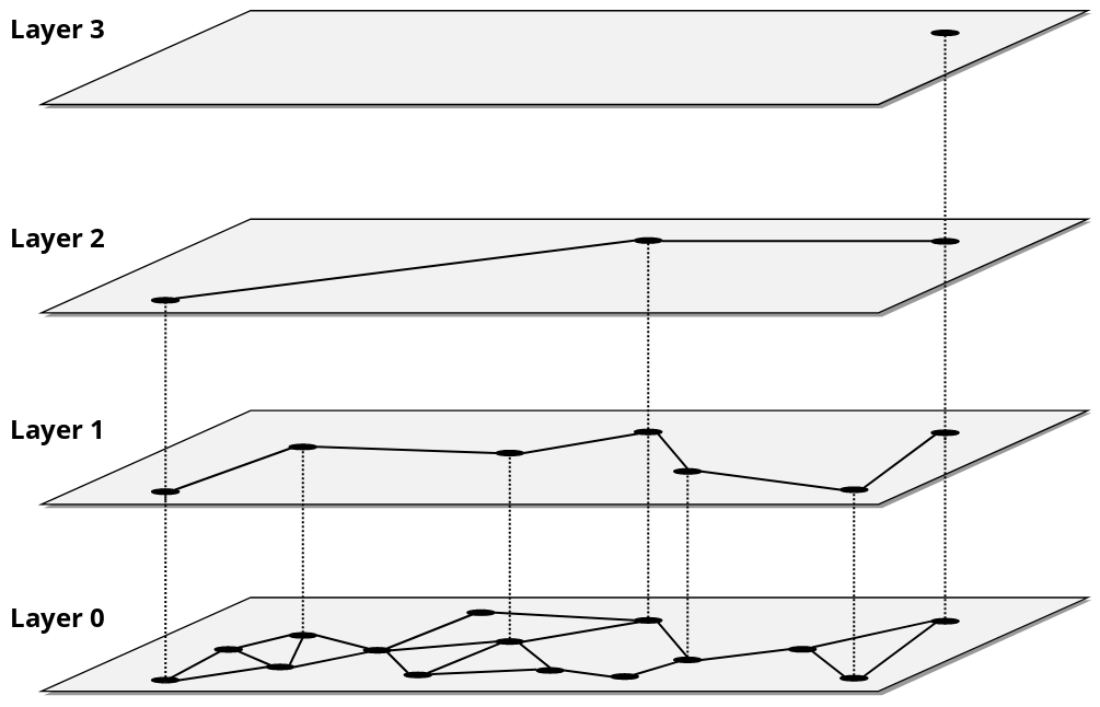
Generally, layer 0 contains all vectors in the database. Additionally, if a node appears in an upper layer, it must also be present in all lower layers. Therefore, the hierarchical structure of HNSW follows the following property:
Regarding the search process, the image below illustrates how it is performed:
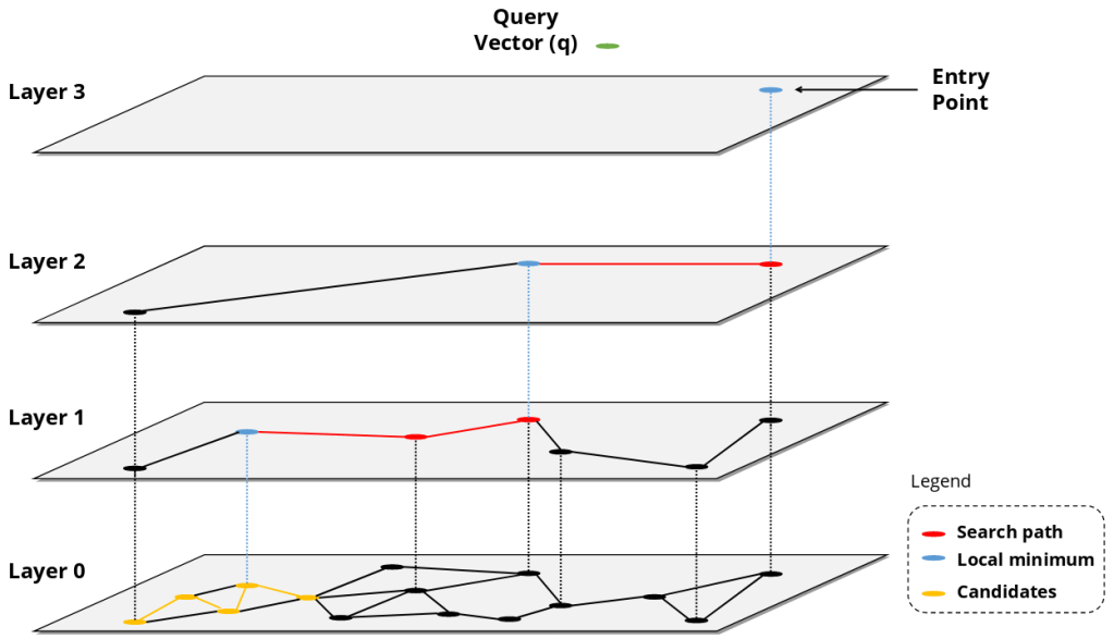
When a query vector is submitted, the search starts from the entry point, the entry node of the hierarchical graph, located at the highest layer. In this example, layer 3 contains only the entry point, so the search moves directly down to layer 2. Once at layer 2, the entry point becomes the current node of the search. From there, the distance between the query vector and each of its neighbors is compared. If any neighbor is closer to the query vector than the current node, the search moves to that neighbor, which then becomes the new current node. This process continues until none of its neighbors is closer to the query than the current node, thus reaching a local minimum at that layer. This node is then used as the entry point for the next layer. The process is repeated until layer 0 is reached.
At layer 0, instead of performing only this greedy navigation until a local minimum is reached, the algorithm performs a broader search around the most promising nodes, exploring multiple candidates. At the end of this process, the closest vectors found are returned as the search result.
How is the Graph Built?
The HNSW algorithm has several hyperparameters, including M, which controls the number of connections between nodes in the graph. Another parameter is , which controls the distribution of nodes across the layers, that is, how quickly the graph layers become sparser. A commonly used choice for is:
During the insertion of a vector into the hierarchical graph, the highest layer to which it will belong is randomly determined. For a vector , this layer, represented by , is calculated as:
where is a value sampled uniformly from the interval (0,1).
But what is the probability that a vector reaches a given layer?
where represents any layer in the hierarchy. Thus, as increases, the probability of a node reaching that layer decreases:
Therefore, the smaller the value of sampled for a vector, the higher the maximum layer that it can reach.
And how is a new vector inserted into the graph? Imagine that we are in the middle of building the graph, which currently has 5 layers, and we want to insert a new vector . Suppose that the maximum layer assigned to this vector is 2, that is, . In the layers above , from to , the algorithm only searches for a good entry point for the next layer, without creating any connections for vector yet.
Suppose we are at one of these layers and is the current node. First, we compute the distance between and , that is, . Then, we compute the distance between and each neighbor of . If any of these neighbors is closer to than , the search moves to that neighbor, which becomes the new node . This process is repeated until none of the neighbors of is closer to than itself, thus reaching a local minimum at that layer. This node then becomes the entry point for the next layer, and the same process is repeated until layer is reached. The pseudocode below represents the process described above:
c ← entryPointfor l = Lmax, Lmax - 1, ..., lx + 1: repeat: v ← closest element to x in neighbors(c) if d(x, v) < d(x, c): c ← v else: break
where is the vector being inserted, is the current node, is a neighbor of , and represents the current layer, located above .
Now, from layer down to layer , the connections for vector are created. To do this, the HNSW algorithm introduces another hyperparameter called efConstruction, whose purpose is to control the number of candidates maintained during the search for the neighbors of . Instead of performing only the greedy search used in the upper layers, the algorithm performs a broader search, maintaining a dynamic list of up to efConstruction candidates. In other words, efConstruction controls how extensively the algorithm explores the existing graph before deciding which nodes will become neighbors of .
How does the candidate search work? Suppose we have a candidate collection and another collection , which maintains the best vectors found so far. Initially, both and contain only the entry point of layer (or layer 2, following the previous example), and they are updated as new vectors are found. From , we remove the candidate that is closest to vector . Now, consider two scenarios:
- In the first scenario, the number of vectors in is still below the allowed limit, that is, . In this case, the unvisited neighbors of are added to both and , allowing the search to continue exploring the graph.
- In the second scenario, has reached its limit, that is, . In this case, we obtain from the vector that is farthest from . Since is the candidate closest to that is still present in , if , the exploration stops. This is because if the best remaining candidate in is already farther from than the worst element in , there are no more promising candidates in to explore. Otherwise, that is, if , the unvisited neighbors of are explored. For each neighbor , if , then is considered promising and added to both and . Since must contain at most
efConstructionelements, if this limit is exceeded, the element in that is farthest from is removed.
The pseudocode below summarizes the candidate search process:
C ← {entryPoint}W ← {entryPoint}V ← {entryPoint}while C ≠ ∅: c ← closest element to x in C remove c from C w ← farthest element from x in W if |W| = efConstruction and d(x, c) > d(x, w): break for each v in neighbors(c): if v not in V: add v to V w ← farthest element from x in W if |W| < efConstruction or d(x, v) < d(x, w): add v to C add v to W if |W| > efConstruction: remove farthest element from x in W
Once we have the best vectors found in , the algorithm does not simply select the vectors closest to , as this could result in redundant connections, that is, connections to vectors located in nearly the same region of the space. To avoid this problem, HNSW uses a heuristic that aims to create more diverse connections. To do so, the candidates in are evaluated in ascending order of distance to . Suppose we have a set of vectors that have already been selected as connections of , where . Now, consider as the next candidate to be evaluated. To determine whether is redundant, we compare its distance to with its distance to each vector already selected in . If there exists any such that
then is rejected. Otherwise, is added to the set as a new connection of .
Another important point is that when a node that already belongs to the graph receives a new connection to node , is also added to the neighbor list of . If this addition causes to exceed the limit of connections allowed at that layer, the neighbor selection process is performed again:
where represents the set of neighbors of node , and SelectNeighbors represents the neighbor selection heuristic described earlier, which is responsible for selecting at most connections.
To summarize, the pseudocode below presents the HNSW graph construction process:
for each x in vectors: # Assign the maximum layer for x lx ← floor(-ln(U) * mL) # Initialize the graph if graph is empty: entryPoint ← x Lmax ← lx continue c ← entryPoint # Greedy search through the upper layers for l = Lmax, Lmax - 1, ..., lx + 1: repeat: v ← closest element to x in neighbors(c, l) if d(x, v) < d(x, c): c ← v else: break # The local minimum becomes the first entry point entryPoints ← {c} # Search and create connections from min(lx, Lmax) down to Layer 0 for l = min(lx, Lmax), ..., 0: W ← SearchLayer(x, entryPoints, efConstruction, l) # Select up to M neighbors using the HNSW heuristic X ← SelectNeighbors(x, W, M) # Create bidirectional connections for each v in X: add v to neighbors(x, l) add x to neighbors(v, l) # Define the maximum number of connections for this layer maxConnections ← 2M if l = 0 else M # Prune v's connections if it exceeds the layer limit if |neighbors(v, l)| > maxConnections: neighbors(v, l) ← SelectNeighbors( v, neighbors(v, l), maxConnections ) # Use all candidates found in this layer # as entry points for the next layer entryPoints ← W # Update the global entry point if x created new upper layers if lx > Lmax: entryPoint ← x Lmax ← lx
It is important to understand that the M and efConstruction hyperparameters have a significant impact on graph construction, and their values should be chosen according to the desired trade-off between search quality, memory usage, and computational cost. In practice, different values can be tested to find a suitable configuration for each use case. Some important points about these hyperparameters are:
M: the higher the value ofM, the more connections each node can have, which can improve graph navigability and, consequently, increase recall, since more paths are available to reach relevant regions of the space. On the other hand, larger values ofMincrease memory usage, index size, and construction and search costs.efConstruction: controls the number of candidates considered during the search for neighbors when building the index. The higher its value, the more extensively the graph is explored before connections are selected, which tends to produce a higher-quality graph and may improve recall. On the other hand, larger values ofefConstructionincrease the computational cost and, consequently, the time required to build the index.
Another important aspect is that, generally, the maximum number of connections per node at layer 0 is 2M, while at the other layers this limit is M. Additionally, the order in which vectors are inserted can influence the final structure of the graph, since each new vector is connected based on the graph that has been built up to that point. Finally, it is worth noting that different implementations of HNSW exist. Although they follow the same general principles presented in this section, libraries and vector databases may adopt their own variations and optimizations for certain aspects of the algorithm.
How is the Search Performed?
To better understand how search works in the HNSW algorithm, we will first explain how it is performed in the upper layers, that is, the layers above layer 0. The purpose of these layers is to enable faster navigation, as they are sparser and allow the algorithm to efficiently traverse the vector space toward a region closer to the query vector.
Suppose we have a query vector and want to find its nearest neighbors. The search starts at the entry point . From there, we compute the distance between and , as well as the distance between and each of its neighbors. If any neighbor of is closer to than itself, that is,
then becomes the new . This process continues until a node is found such that none of its neighbors is closer to than itself, that is,
where represents the set of neighbors of node . Once this local minimum is found, node becomes the entry point for the next layer, and the greedy search is repeated. This process continues until layer 0 is reached.
The pseudocode below summarizes the greedy search performed in the upper layers:
c ← entryPointfor l = Lmax, Lmax - 1, ..., 1: repeat: v ← closest element to q in neighbors(c, l) if d(q, v) < d(q, c): c ← v else: break
And what happens at Layer 0? This is where another HNSW hyperparameter comes into play: efSearch. Instead of following a single greedy path, as in the upper layers, HNSW performs a broader search through the graph, simultaneously maintaining a collection containing up to efSearch of the best vectors found. Basically, the idea is to avoid discarding other promising paths discovered during the search and, consequently, reduce the possibility of getting stuck in a local minimum.
As in the graph construction process, two sets are used during the search: , which contains the promising candidates to be explored, and , which contains the best vectors found. Both sets are initialized with the entry point of layer 0. From , the vector closest to the query vector is selected, that is,
Next, we obtain the neighbors of . First, we check whether the search should continue. Let be the vector farthest from the query . If the candidate is farther from than , that is,
then there are no more promising candidates to explore, and the search is terminated. Otherwise, the unvisited neighbors of are explored. For each neighbor , two scenarios may occur:
- In the first scenario, the set is still below its limit, that is, . In this case, is added to both and .
- In the second scenario, the set has already reached its limit, that is, . In this case, is added to and only if it is closer to than the farthest vector , that is, . Since must contain at most
efSearchelements, whenever a new vector is added and this limit is exceeded, the vector in farthest from is removed.
The pseudocode below summarizes the search process described for layer 0:
C ← {entryPoint}W ← {entryPoint}V ← {entryPoint}while C ≠ ∅: c ← closest element to q in C remove c from C w ← farthest element from q in W if d(q, c) > d(q, w): break for each v in neighbors(c): if v not in V: add v to V w ← farthest element from q in W if |W| < efSearch or d(q, v) < d(q, w): add v to C add v to W if |W| > efSearch: remove farthest element from q in W
Finally, to return the vectors closest to the query vector , the set is sorted according to the distance between each vector and . Then, the first vectors in this ordering are returned as the search result.
The pseudocode below summarizes the entire HNSW search process:
c ← entryPoint# Greedy search through the upper layersfor l = Lmax, Lmax - 1, ..., 1: repeat: v ← closest element to q in neighbors(c, l) if d(q, v) < d(q, c): c ← v else: break# Broader search at Layer 0C ← {c}W ← {c}V ← {c}while C ≠ ∅: c ← closest element to q in C remove c from C w ← farthest element from q in W if d(q, c) > d(q, w): break for each v in neighbors(c, 0): if v not in V: add v to V w ← farthest element from q in W if |W| < efSearch or d(q, v) < d(q, w): add v to C add v to W if |W| > efSearch: remove farthest element from q in W# Return the k nearest neighborssort W by distance to qreturn first k elements of W
It is worth noting that, just like the M and efConstruction hyperparameters used during graph construction, the value of efSearch should also be tuned through experimentation. In general, the higher the efSearch, the higher the search quality and recall tend to be, increasing the chance of finding the true nearest neighbors of the query vector. However, larger values also result in higher query latency and a greater number of distance computations. Additionally, an important property is that:
Finally, it is worth noting that different vector databases may adopt their own variations and optimizations when implementing HNSW search. However, the principles presented in this section represent the foundation upon which these different implementations are built.
Advantages and Disadvantages of HNSW
Compared with exact search, HNSW offers several advantages, including:
- Efficiency: HNSW can significantly reduce search time in large vector datasets by avoiding the need to compare the query vector against every stored vector.
- Scalability: its hierarchical structure enables efficient navigation through the search space even as the number of vectors increases.
- Search speed and quality: HNSW can perform searches significantly faster than exact search while still maintaining high recall when its hyperparameters are properly configured.
However, using HNSW also requires some considerations:
- Higher memory usage: in addition to the vectors themselves, the graph structure and its connections must also be stored. Larger values of
M, for example, increase the number of connections and, consequently, memory usage. - Index construction cost: building an HNSW index requires performing searches and establishing connections for vectors as they are inserted into the graph, making index construction more costly than approaches that do not require building this type of structure.
- Hyperparameter tuning: as shown in the graph construction and search sections, hyperparameters such as
M,efConstruction, andefSearchneed to be adjusted according to the problem. Different configurations affect aspects such as recall, search latency, construction time, and memory usage.
Analyzing HNSW and its Parameters Using FAISS
The goal of this section is to analyze the HNSW algorithm in practice using the FAISS library. To do so, several experiments will be conducted to evaluate the algorithm’s behavior in terms of latency and recall. First, HNSW will be compared with exact search to analyze the speedup it can provide. Next, the index construction process will be analyzed to evaluate how the M and efConstruction hyperparameters affect its behavior. Finally, the search stage will be evaluated, showing how different values of efSearch affect latency and recall.
To perform the experiments, two classes were created: ExactIndex and HNSWIndex. The code for the ExactIndex class is shown below:
import faissimport numpy as npimport timeclass ExactIndex: def __init__( self, number_of_vectors, dimension, number_of_queries ): self.number_of_vectors = number_of_vectors self.dimension = dimension self.number_of_queries = number_of_queries self.index = faiss.IndexFlatL2(self.dimension) rng = np.random.default_rng(seed=123) self.query = rng.random((number_of_queries, dimension), dtype=np.float32) def build_index(self): rng = np.random.default_rng(seed=42) batch_size = 100_000 start_time = time.perf_counter() for batch_start in range(0, self.number_of_vectors, batch_size): size = min(batch_size, self.number_of_vectors - batch_start) vectors = rng.random( (size, self.dimension), dtype=np.float32 ) self.index.add(vectors) latency = time.perf_counter() - start_time return latency def search(self, top_k): start_time = time.perf_counter() _, indices = self.index.search(self.query, top_k) total_latency = time.perf_counter() - start_time avg_latency = total_latency / self.number_of_queries return avg_latency, indices
This class receives in its constructor the number of vectors in the dataset, their dimensionality, and the number of queries to be generated. Additionally, the exact index is created using faiss.IndexFlatL2, with the vector dimensionality passed as an argument. Since this is an experiment, both the dataset and the queries consist of randomly generated vectors. Thus, number_of_queries queries of dimension dimension are generated using NumPy’s rng.random method.
Next, the build_index method is responsible for generating and adding the vectors to the index in batches of 100,000 elements. At the end, the method returns the time required to complete this process. It is worth noting that, unlike HNSW, IndexFlatL2 does not need to build a graph structure to perform searches.
Finally, the search method is responsible for finding the top_k nearest vectors for each query, with top_k provided as an argument. The search is performed using self.index.search, which receives the queries and the number of neighbors to be returned. At the end, the method returns the average latency per query and the indices of the vectors found for each query.
Next, the code for the HNSWIndex class is shown below:
import faissimport numpy as npimport timeclass HNSWIndex: def __init__( self, number_of_vectors, dimension, number_of_queries, M, ef_construction ): self.number_of_vectors = number_of_vectors self.dimension = dimension self.number_of_queries = number_of_queries self.index = faiss.IndexHNSWFlat(dimension, M) self.index.hnsw.efConstruction = ef_construction rng = np.random.default_rng(seed=123) self.query = rng.random((number_of_queries, dimension), dtype=np.float32) def build_index(self): rng = np.random.default_rng(seed=42) batch_size = 100_000 start_time = time.perf_counter() for batch_start in range(0, self.number_of_vectors, batch_size): size = min(batch_size, self.number_of_vectors - batch_start) vectors = rng.random( (size, self.dimension), dtype=np.float32 ) self.index.add(vectors) latency = time.perf_counter() - start_time return latency def search(self, ef_search, top_k): self.index.hnsw.efSearch = ef_search start_time = time.perf_counter() _, indices = self.index.search(self.query, top_k) total_latency = time.perf_counter() - start_time avg_latency = total_latency / self.number_of_queries return avg_latency, indices
Some differences can be observed compared with the ExactIndex class. The constructor of the HNSWIndex class receives the M and efConstruction hyperparameters, which are used during the construction of the HNSW index. The M parameter is passed along with the vector dimensionality when creating the index using faiss.IndexHNSWFlat, while efConstruction is set through self.index.hnsw.efConstruction. The build_index method follows the same structure used in the ExactIndex class, generating and adding vectors to the index in batches. However, in this case, as the vectors are added, the HNSW graph structure is also built. Finally, in the search method, in addition to top_k, the efSearch hyperparameter is received as an argument and set through self.index.hnsw.efSearch. Then, as in the ExactIndex class, self.index.search is used to perform the search. At the end, the method returns the average latency per query and the indices of the vectors found.
Another important aspect of the experiments is the recall calculation, which is used to evaluate the quality of the results returned by HNSW compared with exact search. In this case, Recall@top_k measures the proportion of the neighbors found by exact search that are also found by approximate search. The metric is calculated individually for each query, and the average recall across all queries is then obtained. The method used to perform this calculation is shown below:
def calculate_recall(exact_indices, approximate_indices, top_k): recalls = [] for exact, approximate in zip(exact_indices, approximate_indices): recall = len(set(exact) & set(approximate)) / top_k recalls.append(recall) return sum(recalls) / len(recalls)
The first experiment consists of comparing exact search with the HNSW algorithm. For this purpose, fixed values were defined for the M, efConstruction, and efSearch hyperparameters, without performing any optimization or tuning of these values. The code used to perform the experiment is shown below:
from exact_index import ExactIndexfrom hnsw_index import HNSWIndextop_k = 10number_of_vectors = 1_000_000dimension = 64number_of_queries = 1_000# Exact Indexexact_index = ExactIndex( number_of_vectors=number_of_vectors, dimension=dimension, number_of_queries=number_of_queries)exact_build_latency = exact_index.build_index()exact_search_latency, exact_indices = exact_index.search(top_k)# HNSW IndexM = 16ef_construction = 50ef_search = 100hnsw_index = HNSWIndex( number_of_vectors=number_of_vectors, dimension=dimension, number_of_queries=number_of_queries, M=M, ef_construction=ef_construction)hnsw_build_latency = hnsw_index.build_index()hnsw_search_latency, hnsw_indices = hnsw_index.search(ef_search, top_k)# Resultsrecall = calculate_recall( exact_indices, hnsw_indices, top_k)results = [ { "index": "Exact", "M": None, "ef_construction": None, "ef_search": None, "build_latency_ms": exact_build_latency * 1000, "avg_search_latency_ms": exact_search_latency * 1000, "mean_recall_10": 1.0 }, { "index": "HNSW", "M": M, "ef_construction": ef_construction, "ef_search": ef_search, "build_latency_ms": hnsw_build_latency * 1000, "avg_search_latency_ms": hnsw_search_latency * 1000, "mean_recall_10": recall }]
In this experiment, top_k is set to 10, meaning that the 10 nearest vectors are returned for each query. The dataset consists of 1,000,000 randomly generated 64-dimensional vectors, and the results are evaluated using 1,000 queries. The ExactIndex and HNSWIndex classes are used to execute the two approaches. For each approach, the index construction time and average search latency are recorded. In addition, for HNSW, Recall@10 is calculated using the calculate_recall function presented earlier. Exact search is used as the ground truth and, by definition in this experiment, has a Recall@10 of 1. Therefore, the HNSW recall represents the proportion of neighbors found by exact search that are also retrieved by approximate search.
The table below presents the results of the experiment. Note that constructing the HNSW index was approximately 40 times slower than constructing the exact search index. On the other hand, when searching for the nearest vectors, HNSW was approximately 26 times faster. However, the average Recall@10 was only 26%, indicating that, with the configuration used in this first experiment, a large proportion of the neighbors found by exact search were not retrieved by HNSW. In the following experiments, we will analyze how the HNSW hyperparameters influence these results.
| Index | Build Latency [ms] | AVG Search Latency [ms] | Mean Recall@10 |
| Exact | 302.72 | 1.31 | 1 |
| HNSW | 12,146.5 | 0.05 | 0.26 |
The objective now is to analyze the behavior of the HNSW algorithm as the value of the M hyperparameter increases. It is important to emphasize that this experiment is not intended as a hyperparameter optimization process, but rather to observe how different values of M affect index construction time, search latency, and recall.
The code below presents the experiment. Five values were defined for M: 16, 32, 64, 128, and 256. The values of efConstruction and efSearch were kept fixed at 50 and 100, respectively.
M_values = [16, 32, 64, 128, 256]ef_construction = 50ef_search = 100results = []for M in M_values: hnsw_index = HNSWIndex( number_of_vectors=number_of_vectors, dimension=dimension, number_of_queries=number_of_queries, M=M, ef_construction=ef_construction ) build_latency = hnsw_index.build_index() search_latency, hnsw_indices = hnsw_index.search(ef_search, top_k) recall = calculate_recall( exact_indices, hnsw_indices, top_k ) results.append( { "M": M, "ef_construction": ef_construction, "ef_search": ef_search, "build_latency_ms": build_latency * 1000, "avg_search_latency_ms": search_latency * 1000, "mean_recall@_10": recall } )
The table below presents the results obtained in the experiment. Note that as the value of M increases, the index construction time also becomes higher. A similar behavior can be observed for search, with an increase in average latency. On the other hand, Recall@10 progressively increases, from 26% with to 79% with . Therefore, the results highlight the trade-off associated with the M hyperparameter: in this experiment, larger values resulted in higher recall, but also increased the index construction cost and search latency.
| M | Build Latency [ms] | AVG Search Latency [ms] | Mean Recall@10 |
| 16 | 13,216.3 | 0.04 | 0.26 |
| 32 | 25,566.1 | 0.05 | 0.48 |
| 64 | 38,080.9 | 0.10 | 0.66 |
| 128 | 52,666.0 | 0.13 | 0.75 |
| 256 | 70,854.8 | 0.19 | 0.79 |
The objective now is to analyze the behavior of the HNSW algorithm as the value of the efConstruction hyperparameter increases. The code used is similar to that of the previous experiment, which was performed with the M hyperparameter. Therefore, only the ef_construction_values variable was created, containing the values 50, 100, 150, 200, and 250, which are used in the experiment loop. The values of M and efSearch were kept fixed at 16 and 100, respectively.
The table below presents the results obtained in the experiment. Overall, the index construction time tends to increase as the value of efConstruction increases. The only exception occurs between and , where a reduction in the measured construction time was observed. Nevertheless, the largest efConstruction values resulted in the highest construction times. Regarding search latency, no clear trend was observed as efConstruction increased. This is because efConstruction controls the number of candidates maintained during graph construction and is not directly used during search execution. However, since this hyperparameter influences the structure of the resulting graph, it can indirectly affect search behavior. Finally, Recall@10 improved as efConstruction increased, rising from 26% with to 38% with , and remaining at 38% with . Therefore, in this experiment, larger efConstruction values resulted in a more costly index construction process, but achieved better recall.
| efConstruction | Build Latency [ms] | AVG Search Latency [ms] | Mean Recall@10 |
| 50 | 12,794.0 | 0.04 | 0.26 |
| 100 | 25,157.9 | 0.03 | 0.33 |
| 150 | 37,566.8 | 0.07 | 0.37 |
| 200 | 74,558.2 | 0.03 | 0.38 |
| 250 | 61,926.1 | 0.03 | 0.38 |
Finally, the last experiment analyzes the behavior of HNSW as the value of efSearch increases. The code used differs from that of the previous experiments. Since efSearch is a hyperparameter used during search rather than during index construction, the HNSW graph is built only once and reused across all executions. This makes it possible to observe the effect of different efSearch values on search latency and recall while keeping the graph structure unchanged. The values 100, 200, 300, 400, and 500 were used for efSearch, while M and efConstruction were kept fixed at 16 and 50, respectively. The code used in the experiment is shown below:
M = 16ef_construction = 50ef_search_values = [100, 200, 300, 400, 500]results = []hnsw_index = HNSWIndex( number_of_vectors=number_of_vectors, dimension=dimension, number_of_queries=number_of_queries, M=M, ef_construction=ef_construction)build_latency = hnsw_index.build_index()for ef_search in ef_search_values: search_latency, hnsw_indices = hnsw_index.search(ef_search, top_k) recall = calculate_recall( exact_indices, hnsw_indices, top_k ) results.append( { "M": M, "ef_construction": ef_construction, "ef_search": ef_search, "build_latency_ms": build_latency * 1000, "avg_search_latency_ms": search_latency * 1000, "mean_recall_10": recall } )
The table below presents the results obtained in the experiment. Note that as the value of efSearch increases, search latency also increases. This occurs because larger efSearch values allow a larger set of candidates to be maintained and explored during the search, increasing the number of distance calculations performed. On the other hand, Recall@10 also increases, rising from 26% with to 58% with . Therefore, the results highlight the trade-off associated with efSearch: larger values tend to improve the quality of the results, but increase computational cost and, consequently, search latency.
| efSearch | AVG Search Latency [ms] | Mean Recall@10 |
| 100 | 0.03 | 0.26 |
| 200 | 0.05 | 0.38 |
| 300 | 0.09 | 0.47 |
| 400 | 0.14 | 0.53 |
| 500 | 0.16 | 0.58 |
Therefore, understanding how the HNSW algorithm works and how its hyperparameters affect nearest-neighbor search is essential for using it efficiently. Choosing appropriate values for M, efConstruction, and efSearch makes it possible to establish different trade-offs between index construction time, memory consumption, search latency, and recall, which can have a significant impact on systems that handle large volumes of high-dimensional vectors, such as RAG applications and recommendation systems. In production scenarios, these hyperparameters can be tuned using strategies such as Grid Search or Random Search to find a configuration that meets the specific requirements of the system. After all, there is no single optimal configuration for every use case: the choice depends on the priorities of each application and the desired balance between search quality, speed, index construction cost, and resource consumption.


Leave a comment