
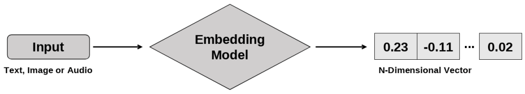
An embedding is a numerical representation of a word, sentence, image, or audio sample in the form of a high-dimensional vector, designed to capture relevant characteristics of the data, such as its semantic meaning.
Embeddings are typically generated by machine learning models trained on large amounts of data. During training, these models learn to organize information within a vector space, where data points with similar characteristics or meanings tend to be positioned close to one another, while less related data points are placed farther apart. For example, in a well-trained text embedding model, words or sentences related to food generally produce vectors that are close to each other, but farther away from vectors associated with sports.
It is important to note that the dimensionality of an embedding corresponds to the number of elements in its vector representation. Different models can generate embeddings with different dimensionalities. For example, the open-source all-MiniLM-L6-v2 model, based on the BERT architecture, produces 384-dimensional vectors, while OpenAI’s text-embedding-3-small model generates 1536-dimensional vectors. In addition, each individual dimension of the vector does not have a human-interpretable meaning. Instead, meaning emerges from the combination of all dimensions, that is, from the vector’s position within the vector space and its relationship to other vectors. In practice, it is these distance and directional relationships between vectors that enable embeddings to represent similarities and differences among data points.
In this post, I’ll cover the following topics:
- Why are embeddings important? Semantic search and RAG
- Using an embedding model
- Visualizing embeddings with PCA
- Measuring similarity with cosine similarity
Why are embeddings important? Semantic search and RAG
Semantic search is an information retrieval technique that aims to understand the meaning, context, and intent behind a user’s query. It differs from traditional keyword-based search, which typically relies on the exact or near-exact occurrence of the searched terms. Although keyword search is effective in many scenarios, it has limitations when it comes to capturing the semantic meaning of content. As a result, relevant documents may fail to be retrieved when they use different words to express the same idea. For example, when searching for “How to learn programming”, a keyword-based search may fail to return documents that use phrases such as “A beginner’s guide to coding”. While both expressions essentially refer to the same topic, they do not share the exact same words. A semantic search system, on the other hand, can identify the similarity between these concepts and retrieve relevant documents even when there is no exact term match.
Semantic search uses embeddings to convert both documents and user queries into numerical vectors that represent their meanings. In general, the process works as follows:
- All documents are processed by an embedding model and converted into numerical vectors. In many real-world applications, these vectors are stored in a vector database, a system specialized in storing, indexing, and efficiently searching high-dimensional vectors. I will discuss vector databases in more detail in a future post.
- When a user submits a query, it is also processed by the same embedding model and converted into a vector.
- Finally, similarity or distance metrics are used to identify which stored vectors are closest to the query vector. The documents associated with those vectors are then returned as search results.
The process described above corresponds to the retrieval stage used in RAG (Retrieval-Augmented Generation) systems. The goal of this approach is to retrieve content from an external source and provide additional context to an LLM. For example, imagine a user asking a question about an internal company procedure. In this scenario, the user’s query can be converted into an embedding vector and compared against the embeddings of documents stored in a vector database. The most semantically relevant content is then retrieved and included in the prompt sent to the model. As a result, the LLM can generate responses based not only on the knowledge acquired during training, but also on information retrieved from the vector database. This typically leads to more grounded responses and reduces the likelihood of hallucinations. I will discuss RAG in more detail in future posts.
Using an embedding model
The goal of this section is to demonstrate, in practice, how a sentence can be transformed into a numerical vector. To do so, we will use two embedding models: all-MiniLM-L6-v2, an open-source model, and OpenAI’s text-embedding-3-small.
The code below demonstrates how to convert the sentence “AI transforms data into intelligence” into an embedding vector using the all-MiniLM-L6-v2 model:
from sentence_transformers import SentenceTransformer

sentence = "AI transforms data into intelligence"

model = SentenceTransformer("sentence-transformers/all-MiniLM-L6-v2")
embedding = model.encode(sentence)

print(f"Embedding: {embedding[:5]}")
print(f"Embedding dimension: {len(embedding)}")
Notice that the model’s full name is passed to the SentenceTransformer class and stored in the model variable. Next, we use the encode method, which is responsible for converting the sentence into a high-dimensional embedding. Finally, we display the first five values of the generated vector, as well as its overall dimensionality, which is 384. The results are shown below:
Embedding: [-0.00760174  0.05849028  0.01688151  0.02850522 -0.01125422]
Embedding dimension: 384
Now, let’s look at the code used to generate an embedding with the text-embedding-3-small model using the same sentence as before:
from openai import OpenAI
from dotenv import load_dotenv
load_dotenv()

client = OpenAI()

sentence = "AI transforms data into intelligence"

response = client.embeddings.create(
    input=sentence,
    model="text-embedding-3-small"
)
embedding = response.data[0].embedding

print(f"Embedding: {embedding[:5]}")
print(f"Embedding dimension: {len(embedding)}")
To run this example, you need an OpenAI API key stored in the OPENAI_API_KEY variable defined in a .env file. To generate embeddings, we use the embeddings.create method, providing the input text and the desired embedding model. The resulting vector can be accessed through response.data[0].embedding. As in the previous example, only the first five dimensions of the vector and its overall dimensionality are displayed, which in this case is 1536. The results are shown below:
Embedding: [-0.0015888214111328125, 0.00969696044921875, 0.03741455078125, 0.006221771240234375, 0.04852294921875]
Embedding dimension: 1536
Visualizing embeddings with PCA
The goal of this section is to illustrate, through a 2D plot, how an embedding model organizes semantically similar concepts within the vector space. As discussed earlier, embedding models generate vectors with hundreds or even thousands of dimensions. Although we can inspect their numerical values, it is difficult to intuitively understand how these vectors are distributed in such a high-dimensional space.
To address this problem, we can use dimensionality reduction techniques. One of the most popular approaches is Principal Component Analysis (PCA), which reduces the number of dimensions while preserving as much relevant information as possible. In simple terms, PCA identifies new directions, called principal components, that capture most of the variation present in the data. The first component represents the direction of greatest variance, while subsequent components capture as much of the remaining variability as possible while remaining orthogonal to the previous components. I will explain how this algorithm works in more detail in a future post.
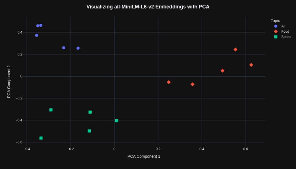
First, we will use the all-MiniLM-L6-v2 model. The code below converts 15 sentences into embeddings, grouped into the topics “AI”, “Food”, and “Sports” (5 sentences for each topic). The result is a 15 × 384 matrix, where 15 corresponds to the total number of sentences and 384 is the dimensionality of the embeddings generated by the model.
from sentence_transformers import SentenceTransformer

model = SentenceTransformer("sentence-transformers/all-MiniLM-L6-v2")

sentences = [
    # AI
    "AI learns from data",
    "Robots can recognize images",
    "Models predict future trends",
    "Chatbots answer user questions",
    "Algorithms improve decision making",

    # Food
    "Pizza tastes very good",
    "Rice cooks very quickly",
    "Fresh fruit is healthy",
    "Soup warms cold days",
    "Bread smells really nice",

    # Sports
    "Players train every day",
    "Football requires teamwork",
    "Basketball improves quick reflexes",
    "Running builds strong endurance",
    "Teams celebrate big victories",
]

embeddings = model.encode(sentences)
Next, PCA was applied using the Scikit-learn (sklearn) library. The parameter n_components=2 was set to reduce the original embeddings to two dimensions, allowing them to be visualized in a 2D plot. The fit_transform method fits the PCA model to the embeddings and returns a new matrix containing the vectors projected onto the first two principal components. Since the dataset contains 15 sentences, the final result is a 15 × 2 matrix.
from sklearn.decomposition import PCA

pca = PCA(n_components=2)
embeddings_2d = pca.fit_transform(embeddings)
Finally, with all vectors reduced to two dimensions, it becomes possible to visualize each data point in a 2D plot. The code below demonstrates how to create this visualization using the Plotly library. However, you can use other libraries of your choice, such as Matplotlib or Seaborn.
from pandas import DataFrame
import plotly.express as px

topics = (
    ["AI"] * 5 +
    ["Food"] * 5 +
    ["Sports"] * 5
)

df = DataFrame({
    "x": embeddings_2d[:, 0],
    "y": embeddings_2d[:, 1],
    "topic": topics,
    "sentence": sentences
})

fig = px.scatter(
    df,
    x="x",
    y="y",
    color="topic",
    symbol="topic",
    hover_data=["sentence"],
)

fig.update_traces(
    marker=dict(size=11)
)

fig.update_layout(
    template="plotly_dark",
    title=dict(
        text="<b>Visualizing all-MiniLM-L6-v2 Embeddings with PCA</b>",
        x=0.5,
        xanchor="center",
        font=dict(size=18)
    ),
    xaxis_title="PCA Component 1",
    yaxis_title="PCA Component 2",
    legend_title="Topic",
    width=1050,
    height=600
)

fig.show()
The resulting plot is shown below. We can observe that the “AI”, “Food”, and “Sports” topics tend to form distinct clusters in the PCA projection. This suggests that the embedding model was able to capture semantic differences between the topics, positioning related concepts close to one another while placing semantically distinct concepts in different regions of the vector space.
Next, we will repeat the same procedure using the text-embedding-3-small model. First, embeddings are generated for the list of sentences. In the code below, each embedding is extracted from the API response using a list comprehension. In the end, we obtain 15 embeddings, each containing 1536 dimensions, which can be represented as a 15 × 1536 matrix.
response = client.embeddings.create(
    input=sentences,
    model="text-embedding-3-small"
)

embeddings = [data.embedding for data in response.data]
The remaining code is very similar to that shown in the previous example. Therefore, the 2D visualization generated by OpenAI’s model is presented below:
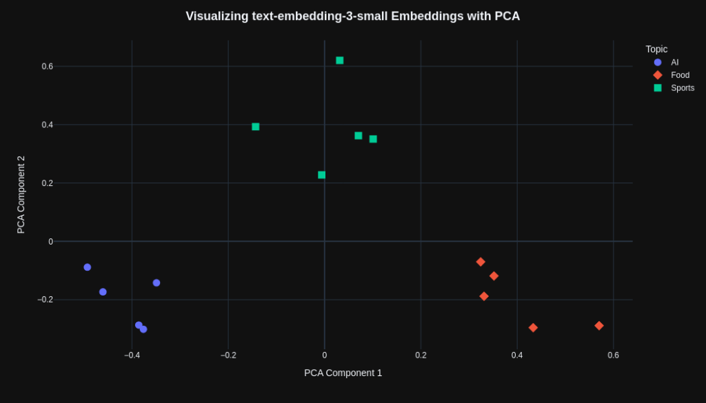
We can observe that both models were able to separate the topics effectively, although the text-embedding-3-small model appears to produce a more visually uniform separation. However, it is not possible to determine which model is superior based solely on these plots, since PCA represents only a projection of the original vectors and may not fully preserve all relationships present in the high-dimensional vector space.
Measuring similarity with cosine similarity
The goal of this section is to identify which sentences are most similar to a target sentence. To do so, we need a metric capable of comparing embeddings and quantifying the degree of similarity between them.
One of the simplest ways to compare vectors is by using Euclidean distance, which measures the distance between two points in vector space. However, this metric is sensitive to vector magnitude. As a result, semantically similar vectors may appear far apart simply because they have different numerical scales. For this reason, one of the most popular metrics for working with embeddings is cosine similarity, which measures the angle between two vectors. If two vectors point in exactly the same direction, the angle between them is 0°, and therefore cos(0) = 1, indicating maximum similarity. If they are orthogonal, the angle is 90° and cos(90) = 0, indicating no alignment. Vectors pointing in opposite directions form an angle of 180°, resulting in cos(180) = -1. This property makes cosine similarity particularly useful for embeddings because it focuses on vector direction while reducing the influence of magnitude. In practice, this allows us to identify conceptually similar documents or sentences even when their embeddings have different scales.
The code below computes the cosine similarity between a target sentence, “Machine learning systems discover hidden relationships in information”, and the 15 sentences used in the previous section.
from sentence_transformers import SentenceTransformer
from sklearn.metrics.pairwise import cosine_similarity
from pandas import DataFrame


model = SentenceTransformer("sentence-transformers/all-MiniLM-L6-v2")

target_sentence = "Machine learning systems discover hidden relationships in information"

sentences = [
    # AI
    "AI learns from data",
    "Robots can recognize images",
    "Models predict future trends",
    "Chatbots answer user questions",
    "Algorithms improve decision making",

    # Food
    "Pizza tastes very good",
    "Rice cooks very quickly",
    "Fresh fruit is healthy",
    "Soup warms cold days",
    "Bread smells really nice",

    # Sports
    "Players train every day",
    "Football requires teamwork",
    "Basketball improves quick reflexes",
    "Running builds strong endurance",
    "Teams celebrate big victories",
]

target_embedding = model.encode(target_sentence)
embeddings = model.encode(sentences)

similarities = cosine_similarity([target_embedding], embeddings)[0]

topics = (
    ["AI"] * 5 +
    ["Food"] * 5 +
    ["Sports"] * 5
)

df = DataFrame({
    "topic": topics,
    "sentence": sentences,
    "cosine_similarity": similarities
}).sort_values("cosine_similarity", ascending=False)
The all-MiniLM-L6-v2 model was used to generate the embeddings. Notice that both the target sentence and the 15 sentences are converted into embeddings before the comparison takes place. Next, the cosine_similarity function is used to compute the similarity between the target sentence embedding and the vectors generated for each sentence in the list. Finally, the results are organized into a DataFrame containing three columns: the topic associated with each sentence, the sentence itself, and the computed cosine similarity score. This DataFrame is then sorted by the highest similarity scores.
The table below illustrates how the DataFrame is organized. We can observe that four of the five sentences from the AI topic appear among the most similar to the target sentence, indicating that the model was able to capture the semantic relationship between these concepts. However, the sentence “Players train every day”, from the Sports topic, achieved a higher similarity score than “Chatbots answer user questions”, from the AI topic.
| topic | sentence | cosine_similarity |
| AI | AI learns from data | 0.487907 |
| AI | Algorithms improve decision making | 0.302863 |
| AI | Robots can recognize images | 0.278075 |
| AI | Models predict future trends | 0.271455 |
| Sports | Players train every day | 0.109714 |
| AI | Chatbots answer user questions | 0.091661 |
| Food | Bread smells really nice | 0.078077 |
| Food | Soup warms cold days | 0.045030 |
| Food | Fresh fruit is healthy | 0.042361 |
| Food | Pizza tastes very good | 0.035914 |
| Sports | Teams celebrate big victories | 0.025817 |
| Food | Rice cooks very quickly | 0.015671 |
| Sports | Running builds strong endurance | 0.002094 |
| Sports | Basketball improves quick reflexes | -0.003989 |
| Sports | Football requires teamwork | -0.010182 |
Finally, the similarity scores will be computed using the text-embedding-3-small model. The procedure is very similar to the one presented earlier, differing only in how the embeddings for the target sentence and the list of sentences are generated. The code is shown below:
target_response = client.embeddings.create(
    input=target_sentence,
    model="text-embedding-3-small"
)
target_embedding = target_response.data[0].embedding

response = client.embeddings.create(
    input=sentences,
    model="text-embedding-3-small"
)
embeddings = [data.embedding for data in response.data]
The table below presents the similarity scores computed for each sentence. Unlike the previous model, all sentences related to the AI topic appear among the most similar to the target sentence. This result is more consistent with our intuitive expectations, since the target sentence itself also addresses concepts related to machine learning and data analysis.
| topic | sentence | cosine_similarity |
| AI | AI learns from data | 0.506395 |
| AI | Algorithms improve decision making | 0.486875 |
| AI | Models predict future trends | 0.362968 |
| AI | Robots can recognize images | 0.322411 |
| AI | Chatbots answer user questions | 0.236478 |
| Sports | Players train every day | 0.159671 |
| Sports | Football requires teamwork | 0.119314 |
| Sports | Teams celebrate big victories | 0.090849 |
| Sports | Running builds strong endurance | 0.079309 |
| Sports | Basketball improves quick reflexes | 0.069862 |
| Food | Fresh fruit is healthy | 0.056209 |
| Food | Pizza tastes very good | 0.055679 |
| Food | Bread smells really nice | 0.045437 |
| Food | Soup warms cold days | 0.033070 |
| Food | Rice cooks very quickly | 0.018145 |
When comparing the two models, the text-embedding-3-small produced a ranking that was more aligned with expectations in this example than the all-MiniLM-L6-v2. Nevertheless, both models were able to capture the semantic relationships present in the sentences effectively. Therefore, it is important to evaluate which embedding model is most appropriate for a given use case, taking into account factors such as performance, latency, cost, and application requirements.

Leave a comment